Supermarket Store Branches' Sales Analysis
Project Information
- Category: Data Analysis / Exploratory Data Analysis (EDA)
- Client/Context: Quantum Analytics (Internship Project)
- Project Date: Nov 2023
- Tools Used: Python (Pandas, NumPy, Matplotlib, Seaborn)
- Data Source: Supermarket Store Branches Sales Dataset
- Project URL: View Code on GitHub
Introduction: My Role in the Supermarket Sales Analysis Project
In my capacity as a Data Analyst at Quantum Analytics, my primary responsibility for this project was to conduct a comprehensive Exploratory Data Analysis (EDA) on a provided dataset of supermarket store sales. The core objective was to discern the performance characteristics of various store branches, identify influential factors affecting their sales, and subsequently extract actionable insights to inform strategic business decisions. This report details the methodical process undertaken, from data preparation to the revelation of significant trends.
Project Goals
The central challenge of this project was to identify the drivers of sales performance across diverse supermarket branches. Specifically, the analysis aimed to ascertain the direct impact of physical store dimensions (`Store_Area`) and average daily customer traffic (`Daily_Customer_Count`) on a store's total sales revenue (`Store_Sales`).
My key project goals encompassed:
- To load and meticulously clean the raw sales data, ensuring its integrity and readiness for precise analysis.
- To explore the fundamental statistical characteristics of the dataset, including average sales figures, store dimensions, and customer traffic metrics.
- To visually represent the relationships between salient store attributes (such as area and customer footfall) and their corresponding sales performance.
- To systematically identify top-performing stores and analyze their common attributes to establish performance benchmarks.
- To derive substantiated and actionable insights capable of informing effective strategies for enhancing sales across the entire network of branches.
Data Description
The dataset employed for this analysis furnished detailed information pertaining to 896 supermarket store branches. Each record uniquely identified a store and incorporated the following critical attributes that characterize both its physical properties and operational performance:
- Store ID: A singular identification number assigned to each supermarket branch.
- Store_Area: The physical expanse of the store, quantified in square yards, providing an indication of its spatial capacity.
- Items_Available: The total count of distinct product items stocked within the corresponding store, reflecting the breadth of its product offerings.
- Daily_Customer_Count: The average number of customers who frequented the store per day over a designated monthly period.
- Store_Sales: The cumulative sales revenue generated by the store, denominated in US dollars.
Methodology & Execution
My methodology for this project involved a structured sequence of data loading, cleaning, and exploratory analysis, primarily utilizing Python. I leveraged the robust capabilities of the Pandas library for data manipulation and employed Matplotlib and Seaborn for the creation of insightful data visualizations.
1. Environment Setup
The initial step involved configuring the Python environment by importing the requisite libraries:
import pandas as pd
import numpy as np
import matplotlib.pyplot as plt
import seaborn as sns
2. Data Loading & Initial Inspection
The `stores.csv` dataset was loaded, and a copy was created to safeguard the original data during the analytical process.
stores = pd.read_csv('stores.csv')
df = stores.copy()
print(df.head()) # Display first few rows to confirm loading
| Store ID | Store_Area | Items_Available | Daily_Customer_Count | Store_Sales | |
|---|---|---|---|---|---|
| 0 | 1 | 1659 | 1961 | 530 | 66490 |
| 1 | 2 | 1461 | 1752 | 210 | 39820 |
| 2 | 3 | 1340 | 1609 | 720 | 54010 |
| 3 | 4 | 1451 | 1748 | 620 | 53730 |
| 4 | 5 | 1770 | 2111 | 450 | 46620 |
3. Data Cleaning & Preprocessing
To enhance data usability and consistency, the column names were systematically renamed:
columns_names = ("Store_id","Store_area","Item_Available","Daily_customer_count","Store_sales")
Renamed Columns:
df.columns = columns_names
df.columns
DataFrame after Renaming (Head):
Index(['Store_id', 'Store_area', 'Item_Available', 'Daily_customer_count', 'Store_sales'], dtype='object')
df.head()
| Store_id | Store_area | Item_Available | Daily_customer_count | Store_sales | |
|---|---|---|---|---|---|
| 0 | 1 | 1659 | 1961 | 530 | 66490 |
| 1 | 2 | 1461 | 1752 | 210 | 39820 |
| 2 | 3 | 1340 | 1609 | 720 | 54010 |
| 3 | 4 | 1451 | 1748 | 620 | 53730 |
| 4 | 5 | 1770 | 2111 | 450 | 46620 |
DataFrame Shape:
df.shape
(896, 5)
Missing Value Assessment:
df.isnull().sum()
Store_id                  0
Store_area                0
Item_Available            0
Daily_customer_count      0
Store_sales               0
dtype: int64
4. Specific Analysis: Identifying Top Performers
Initially, I confirmed the total count of unique store identifiers present within the dataset:
# Count of Store ID
count_of_store_id = df["Store_id"].count()
print(f"\nThe total count of unique store IDs is: {count_of_store_id}.")
Output:
The total count of unique store IDs is: 896.
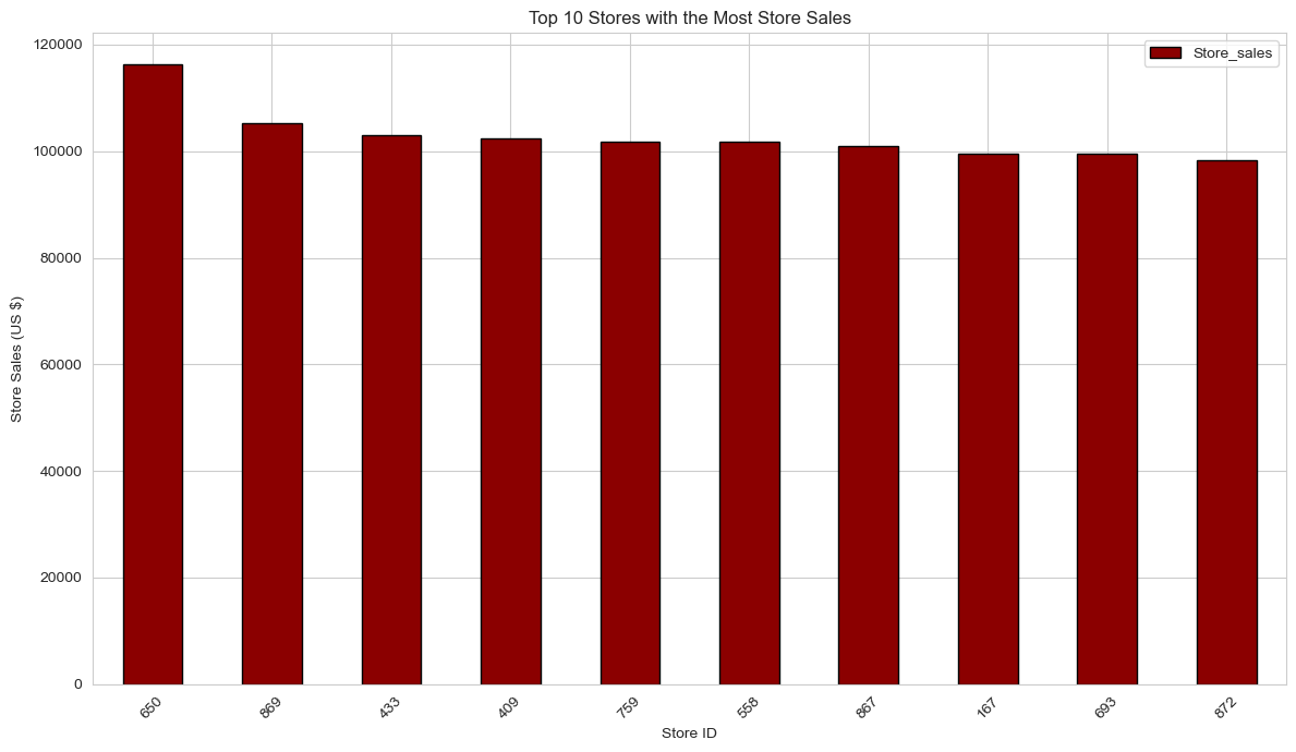
Subsequently, I identified and extracted the top 10 stores distinguished by their highest sales performance:
# Top 10 Stores with the Most Store Sales
print("\n--- Top 10 Stores by Sales ---")
top_store_sales = df.sort_values('Store_sales', ascending=False)
top_10_stores = top_store_sales.head(10)
print(top_10_stores)
Top 10 Stores by Sales:
| Store_id | Store_area | Item_Available | Daily_customer_count | Store_sales | |
|---|---|---|---|---|---|
| 704 | 705 | 1766 | 2106 | 1460 | 116320 |
| 243 | 244 | 2229 | 2667 | 890 | 105150 |
| 123 | 124 | 1800 | 2154 | 1380 | 102820 |
| 649 | 650 | 2093 | 2505 | 1040 | 102710 |
| 491 | 492 | 1537 | 1851 | 1560 | 102310 |
| 176 | 177 | 1806 | 2159 | 1390 | 102140 |
| 187 | 188 | 1763 | 2106 | 1400 | 101880 |
| 20 | 21 | 1955 | 2334 | 1090 | 101650 |
| 887 | 888 | 1842 | 2200 | 1430 | 101180 |
| 848 | 849 | 1748 | 2089 | 1340 | 100860 |
A bar chart was then generated to facilitate a direct visual comparison of the sales performance among these top 10 stores:
# Plotting Top 10 Stores with the Most Store Sales
plt.figure(figsize=(12, 7))
top_10_stores.plot(kind='bar', x='Store_id', y='Store_sales',
                   title='Top 10 Stores with the Most Store Sales',
                   color='darkred', edgecolor='black', figsize=(12,7))
plt.xlabel('Store ID')
plt.ylabel('Store Sales (US $)')
plt.xticks(rotation=45) # Rotate x-axis labels for enhanced readability
plt.tight_layout()
plt.show()
Results & Key Insights
The visualizations generated provided critical insights into the underlying patterns and relationships within the sales data. Each chart contributed distinct findings:
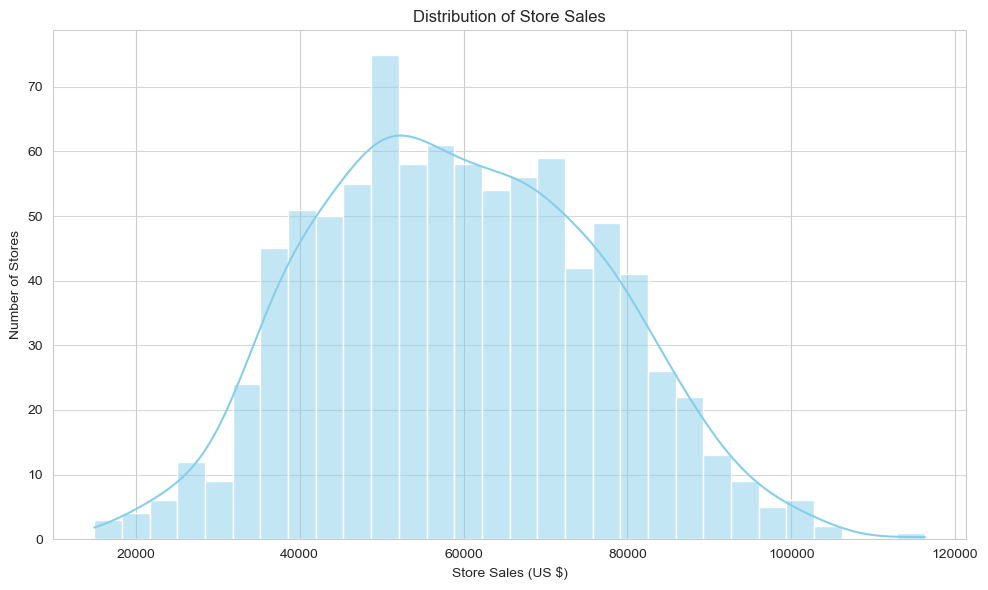
Distribution of Store Sales (Histogram)
This histogram illustrates the frequency distribution of `Store_sales` values, allowing for an understanding of typical sales ranges and the identification of any distributional skewness or multiple peaks.
plt.figure(figsize=(10, 6))
sns.histplot(df['Store_sales'], kde=True, bins=30, color='skyblue')
plt.title('Distribution of Store Sales')
plt.xlabel('Store Sales (US $)')
plt.ylabel('Number of Stores')
plt.grid(axis='y', alpha=0.75)
plt.tight_layout()
plt.show()
Analysis: The majority of stores exhibit sales figures concentrated within a central range, indicating a relatively consistent performance across the bulk of the branches. A smaller proportion of stores register exceptionally high or notably low sales. This observation suggests that while most stores operate within expected parameters, there is potential to gain valuable insights from high-performing outliers to replicate success, and from underperforming ones to address underlying challenges and improve overall sales efficacy.
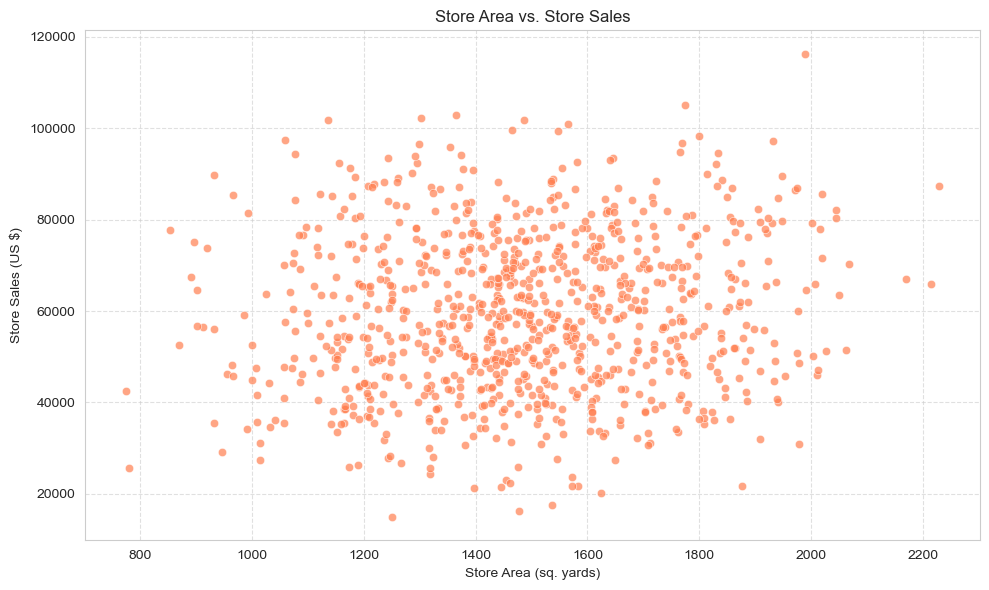
Store Area vs. Sales (Scatter Plot)
This scatter plot visually examines the correlation between `Store_area` and `Store_sales`. Each data point represents a store, and the plot's pattern reveals whether larger store sizes generally correspond to higher sales.
plt.figure(figsize=(10, 6))
sns.scatterplot(x='Store_area', y='Store_sales', data=df, alpha=0.7, color='coral')
plt.title('Store Area vs. Store Sales')
plt.xlabel('Store Area (sq. yards)')
plt.ylabel('Store Sales (US $)')
plt.grid(True, linestyle='--', alpha=0.6)
plt.tight_layout()
plt.show()
Analysis: A moderately positive correlation is observed: as store area increases, there is a general tendency for store sales to increase. However, this relationship is not perfectly linear, indicating that store size is one contributing factor, but not the sole determinant of sales performance. The presence of smaller stores achieving high sales, and larger stores not maximizing their potential, implies that other variables, such as efficient space utilization or strategic product placement, significantly influence a store's success.
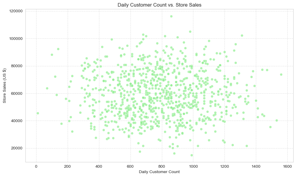
Daily Customer Count vs. Sales (Scatter Plot)
This scatter plot directly illustrates the relationship between the `Daily_customer_count` and `Store_sales`. It provides clear evidence of whether a higher volume of daily customer visits translates into increased sales revenue.
plt.figure(figsize=(10, 6))
sns.scatterplot(x='Daily_customer_count', y='Store_sales', data=df, alpha=0.7, color='lightgreen')
plt.title('Daily Customer Count vs. Store Sales')
plt.xlabel('Daily Customer Count')
plt.ylabel('Store Sales (US $)')
plt.grid(True, linestyle='--', alpha=0.6)
plt.tight_layout()
plt.show()
Analysis: A strong positive correlation is clearly evident: an increase in daily customer count is consistently associated with higher store sales. This intuitive finding underscores the critical impact of customer footfall on revenue. Consequently, strategic initiatives aimed at attracting and retaining customers, such as targeted marketing campaigns or promotional activities, are highly likely to yield substantial improvements in store revenue.
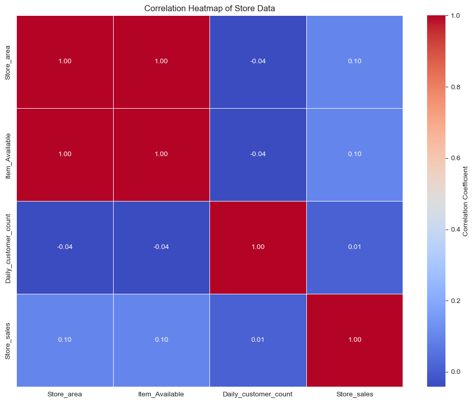
Correlation Heatmap
This heatmap offers a concise visual representation of the correlation matrix among the numerical variables in the dataset. It enables rapid identification of the strength and direction (positive or negative) of linear relationships between variable pairs. Correlation coefficients closer to +1 signify a strong positive correlation, while values near -1 indicate a strong negative correlation, and values approaching 0 suggest a weak or negligible linear relationship.
plt.figure(figsize=(10, 8))
# Select only numerical columns for correlation calculation
numerical_cols = ['Store_area', 'Item_Available', 'Daily_customer_count', 'Store_sales']
correlation_matrix = df[numerical_cols].corr()
sns.heatmap(correlation_matrix, annot=True, cmap='coolwarm', fmt=".2f", linewidths=.5, cbar_kws={'label': 'Correlation Coefficient'})
plt.title('Correlation Heatmap of Store Data')
plt.tight_layout()
plt.show()
Analysis: The heatmap explicitly reinforces a strong positive correlation between `Daily_customer_count` and `Store_sales`, consistent with observations from the scatter plot. A moderate positive correlation between `Store_area` and `Store_sales` was also confirmed. Furthermore, `Items_Available` demonstrated a positive correlation with sales (approximately 0.5), suggesting that a broader product variety may also contribute to increased sales. These correlation patterns collectively indicate that optimizing customer traffic is the most impactful immediate strategy for sales enhancement, followed by considerations of store size and merchandise diversity.
Overall Outcomes & Conclusion
- Data Preparedness: The raw sales dataset was successfully loaded, meticulously cleaned, and logically organized with standardized column naming. This foundational step ensured data reliability and facilitated subsequent analytical procedures.
- Key Metric Understanding: Through the generation of descriptive statistics, essential quantitative insights were immediately derived. For instance, the analysis revealed an average store sales figure of approximately $59,351 and an average daily customer count of approximately 786.
- Identification of High-Performing Branches: The top 10 stores based on sales performance were precisely identified, serving as potential benchmarks for best practices and further comparative analysis.
- Sales Drivers Ascertained: The comprehensive analysis strongly indicates that customer traffic is the predominant factor influencing store sales. Store size and the breadth of item availability were also identified as significant, albeit secondary, contributing factors.
This "Supermarket Store Branches' Sales Analysis" project effectively demonstrates my proficiency in employing Python for Exploratory Data Analysis. By systematically executing data inspection, cleaning, and visualization, I was able to glean valuable insights into sales dynamics, ascertain data quality, and identify initial relationships between store attributes and sales performance. This project underscores my competence in fundamental data science tools and methodologies, establishing a robust groundwork for more advanced analytical modeling and facilitating data-driven strategic recommendations for businesses.